My Journey to Music-Speech with Deep Learning (Part 1) - Music Generation with LSTM
INTRODUCTION
Neural networks are widely used in different areas such as cancer detection, autonomous cars, recommendation systems. With the Andrej Karpathy’s post which is about RNN, generative Deep Learning (DL) become popular among different areas. With this post, researcher mostly start to focus to text generation for fun. However as you can see in the comments, some researcher give idea about music generation with Deep Learning.
Also, we can see great efforts in this area like Google’s Magenta and Aiva which is Luxembourg based startup for music generation. Especially, Aiva’s musics are amazing and their contents are registered under the France and Luxembourg authors’ right society (SACEM).
With this impression, I want to start my own journey to this area. And this blog-post explains my first step to this journey.
LSTM
Colah’s post gives great insight about LSTM. Also, I will try to give information about LSTM.
Traditional neural networks can not remember past information. They can only process current information. As you can think, if you can not remember past information, probably you can not even produce meaningful sentences. Recurrent Neural Network(RNN) solve this problem thanks to recurrent connection via loops at nodes. However, Vanilla RNN has another problem called as vanishing gradient. At this point, you can ask what is gradient and why this problem is big deal. Let me explain these concepts in one paragraph.

Gradient is a fancy words for slope of line(for 2D space) a.k.a derivative. We use gradient to find minimum points of the function. I think this quote will give intuitive explanation: The gradient will act like a compass and always point us downhill. To compute it, we will need to differentiate our error function. We can say that, gradient descent is a way to minimize objective function. (Gradient descent is an optimization algorithm that minimizes functions.) This optimization technique is based on repetition. For the initialization, model guess some parameter and according to gradient (derivative) of objective function, model updates their parameter. As you expect, its usage for Deep Learning comes with the loss(cost) function. Most of the time, our aim is minimize the loss(cost) function for DL models. Gradient based methods learn a parameter’s value (weights of node or biases) by understanding how a small change in this parameter’s value will affect the outputs of the network. When vanishing gradient problem occurs, gradient of early layers of the model’s parameters’ become very small. Thus, DL model can not find the better value for parameter effectively to decrease loss function with find the minimum point of line thanks to gradient.
You can check this excellent resource for mathematical and graphical explanation of gradient descent:
.mid Files
.mid files include midi datas. Midi is an abbreviation for Musical Instrument Digital Interface.
This type of files do not include actual audio as opposed to .mp3 and .wav. .mid files explain what notes are played and how long or loud each note should be.
.mid files can include different instruments such as flute, _obua ,muted bass. However, we are using just piano part of .mid files for this post.
Framework
I have used Keras as a Deep Learning framework with Tensorflow backend. Because, it is easier than pure Tensorflow API for me.
Music21
Music21 is Python-based toolkit for computer-aided musicology. It is developed by MIT researchers and community.
People use music21 to answer questions from musicology using computers, to study large datasets of music, to generate musical examples, to teach fundamentals of music theory, to edit musical notation, study music and the brain, and to compose music (both algorithmically and directly).
I have used music21 toolkit to read .mid file and extract informations as notes, durations and offsets. Also, I have created matrix from these informations via this toolkit. Furthermore, I have used this toolkit to create new .mid file from generated matrix.
Code Part
When you want to feed your deep learning model, you need input as matrix format. So that, I should convert .midi files to matrix format. For this process
- Read midi file and extract information about notes, durations and offsets.
- Convert these informations to matrix.
NOTE: You can find full code in my GitHub repository. I will provide snippets from code for better understanding in this post.
Let’s Start!
- Firstly, we need extract information from .mid file. We need three information which are notes, duration of notes and offset of notes. (Duration represent the how long played, offset represent the when played) Also, I need just piano part’s information.
midi = music21.converter.parse(filename)
notes_to_parse = None

parts = music21.instrument.partitionByInstrument(midi)

instrument_names = []

try:
    for instrument in parts: # Learn names of instruments.
        name = (str(instrument).split(' ')[-1])[:-1]
        instrument_names.append(name)

except TypeError:
    print ('Type is not iterable.')
    return None

    # Just take piano part. For the future works, we can use different instrument.
    try:
        piano_index = instrument_names.index('Piano')
    except ValueError:
        print ('%s have not any Piano part' %(filename))
        return None


    notes_to_parse = parts.parts[piano_index].recurse()

    duration_piano = float(check_float((str(notes_to_parse._getDuration()).split(' ')[-1])[:-1]))

    durations = []
    notes = []
    offsets = []

    for element in notes_to_parse:
        if isinstance(element, note.Note): # If it is single note
            notes.append(note_to_int(str(element.pitch))) # Append note's integer value to "notes" list.
            duration = str(element.duration)[27:-1]
            durations.append(check_float(duration))
            offsets.append(element.offset)

        elif isinstance(element, chord.Chord): # If it is chord
            notes.append('.'.join(str(note_to_int(str(n)))
                                  for n in element.pitches))
            duration = str(element.duration)[27:-1]
            durations.append(check_float(duration))
            offsets.append(element.offset)
Now we have three different list which are for
- Notes
- Duration
- Offset
Note: I have convert note’s representation from letter to integer. This process has done by note_to_int function.
def note_to_int(note): # converts the note's letter to pitch value which is integer form.

    note_base_name = ['C', 'C#', 'D', 'D#', 'E', 'F', 'F#', 'G', 'G#', 'A', 'A#', 'B']
    if ('#-' in note):
        first_letter = note[0]
        base_value = note_base_name.index(first_letter)
        octave = note[3]
        value = base_value + 12*(int(octave)-(-1))

    elif ('#' in note):
        first_letter = note[0]
        base_value = note_base_name.index(first_letter)
        octave = note[2]
        value = base_value + 12*(int(octave)-(-1))

    elif ('-' in note):
        first_letter = note[0]
        base_value = note_base_name.index(first_letter)
        octave = note[2]
        value = base_value + 12*(int(octave)-(-1))

    else:
        first_letter = note[0]
        base_val = note_base_name.index(first_letter)
        octave = note[1]
        value = base_val + 12*(int(octave)-(-1))

    return value
Create matrix to represent midi file with using information which comes from previous lists.
- Create matrix with random uniform values.
- X-axis of this matrix will represent time (duration and offset) and Y-axis will represent the frequency (pitch a.k.a notes). This matrix will be like spectogram.
- We have 128 different pitch value, so that length of matrix’s Y-axis will be equal to 128. For the time representation, I have choosen 0.25 note length as minimum value. Because, most notes is multiplication of 0.25.
try: last_offset = int(offsets[-1]) except IndexError: print ('Index Error') return (None, None, None) total_offset_axis = last_offset * 4 + (8 * 4) our_matrix = np.random.uniform(min_value, lower_first, (128, int(total_offset_axis))) -
Read lists and extract information to modify matrix to represent midi. I have spent too much time to determine how distunguish between a long note and many short notes. According to my trials, best method is represent a long note with bigger value at first occurence’s offset, smaller value at continuation’s offset. For instance, C4 with duration 0.75 will be represented as 1.0-0.5-0.5, three 0.25 C4 will be represented as 1.0-1.0-1.0.
-
However, for better generalization, we can add some randomness to these values. But, in this codes, I have not done that. (If you want to this, for instance you can change lower_first to 0.1, lower_second to 0.4, upper_first to 0.6, upper_second to 0.8)
  for (note, duration, offset) in zip(notes, durations, offsets):
      how_many = int(float(duration)/0.25) # indicates time duration for single note.

      # Define difference between single and double note.
      # I have choose the value for first touch, the another value for continuation.
      # Lets make it randomize

      # I choose to use uniform distrubition. Maybe, you can use another distrubition like Gaussian.

      first_touch = np.random.uniform(upper_second, max_value, 1)
      continuation = np.random.uniform(lower_second, upper_first, 1)

      if ('.' not in str(note)): # It is not chord. Single note.
          our_matrix[note, int(offset * 4)] = first_touch
          our_matrix[note, int((offset * 4) + 1) : int((offset * 4) + how_many)] = continuation

      else: # For chord
          chord_notes_str = [note for note in note.split('.')]
          chord_notes_float = list(map(int, chord_notes_str)) # Take notes in chord one by one

          for chord_note_float in chord_notes_float:
              our_matrix[chord_note_float, int(offset * 4)] = first_touch
              our_matrix[chord_note_float, int((offset * 4) + 1) : int((offset * 4) + how_many)] = continuation
Build Database
Now, we can create dataset from .mid file with these functions. For this post, I have used great composer Schumann .mid files.
Firstly, I have convert all midi file to matrix one by one and append single midi’s matrix to list of cumulative matrix. However, this matrix is instance of list format and we can not use this format for array manipulation. So that, I have convert the list to numpy array and save this array which includes Schumann’s .mid to .npy file to use easily with another platform and later use.
Note: You can use a zip file which includes your inputs as .mid format. The code will extract zip and create numpy array and .npy file. You can find commented version of this code block in my github repo. I will not share it in this post.
# Build database

database_npy = 'midis_array_schumann.npy'
my_file_database_npy = Path("./database_npy/" + database_npy )


if my_file_database_npy.is_file():
    midis_array = np.load(my_file_database_npy)

else:
    print (os.getcwd())
    root_dir = ('./midi_files')
    all_midi_paths = glob.glob(os.path.join(root_dir,'classic/schumann/*mid'))
    print (all_midi_paths)
    matrix_of_all_midis = []

    # All midi have to be in same shape.

    for single_midi_path in all_midi_paths:
        print (single_midi_path)
        matrix_of_single_midi = midi_to_matrix(single_midi_path, length=250)
        if (matrix_of_single_midi is not None):
            matrix_of_all_midis.append(matrix_of_single_midi)
            print (matrix_of_single_midi.shape)
    midis_array = np.asarray(matrix_of_all_midis)
    np.save(my_file_database_npy, midis_array)
Transform Database
When you load .npy file to numpy array, your array’s shape will be (# of file, # of freq, # of time in a single file). You can not use this type of array directly. So that, we have to modify this data to use with LSTM.
- Firstly, I will convert to (# of file, # of time in a single file, # of freq)
midis_array = np.transpose(midis_array_raw, (0, 2, 1))
midis_array = np.asarray(midis_array)
- Secondly, convert to (# of freq, # of file * # of time in a single file)
midis_array = np.reshape(midis_array,(-1,128))
midis_array.shape
- Finally, create 2 different array for training. First one will be used to predict next array, and second one will represent true array. Weights of layer of LSTM will be based on error between prediction array which is based on first array and true array. With gradient descent, model update each layer to decrease this error.
max_len = 18 # how many column will take account to predict next column.
step = 1 # step size.

previous_full = []
predicted_full = []

for i in range (0, midis_array.shape[0]-max_len, step):
    prev = midis_array[i:i+max_len,...] # take max_len column.
    pred = midis_array[i+max_len,...] # take (max_len)th column.
    previous_full.append(prev)
    predicted_full.append(pred)

Now we can build our deep learning model with KERAS Api. I have used 3 LSTM layer and 2 Dense Layer. Also, model’s final activation function is softmax because we want to output which is between 0 and 1. Also, I have used LeakyReLU and Dropout layers to get rid of gradient problem.
Build our Deep Learning Architecture
# Build our Deep Learning Architecture

from keras import layers
from keras import models
import keras
from keras.models import Model
import tensorflow as tf
from keras.layers.advanced_activations import *


midi_shape = (max_len, 128)

input_midi = keras.Input(midi_shape)

x = layers.LSTM(1024, return_sequences=True, unit_forget_bias=True)(input_midi)
x = layers.LeakyReLU()(x)
x = layers.BatchNormalization() (x)
x = layers.Dropout(0.3)(x)

# compute importance for each step
attention = layers.Dense(1, activation='tanh')(x)
attention = layers.Flatten()(attention)
attention = layers.Activation('softmax')(attention)
attention = layers.RepeatVector(1024)(attention)
attention = layers.Permute([2, 1])(attention)

multiplied = layers.Multiply()([x, attention])
sent_representation = layers.Dense(512)(multiplied)


x = layers.Dense(512)(sent_representation)
x = layers.LeakyReLU()(x)
x = layers.BatchNormalization() (x)
x = layers.Dropout(0.22)(x)

x = layers.LSTM(512, return_sequences=True, unit_forget_bias=True)(x)
x = layers.LeakyReLU()(x)
x = layers.BatchNormalization() (x)
x = layers.Dropout(0.22)(x)


# compute importance for each step
attention = layers.Dense(1, activation='tanh')(x)
attention = layers.Flatten()(attention)
attention = layers.Activation('softmax')(attention)
attention = layers.RepeatVector(512)(attention)
attention = layers.Permute([2, 1])(attention)

multiplied = layers.Multiply()([x, attention])
sent_representation = layers.Dense(256)(multiplied)


x = layers.Dense(256)(sent_representation)
x = layers.LeakyReLU()(x)
x = layers.BatchNormalization() (x)
x = layers.Dropout(0.22)(x)


x = layers.LSTM(128, unit_forget_bias=True)(x)
x = layers.LeakyReLU()(x)
x = layers.BatchNormalization() (x)
x = layers.Dropout(0.22)(x)


x = layers.Dense(128, activation='softmax')(x)

model = Model(input_midi, x)
We have used LSTM, LeakyReLU, BatchNormalization, Dropout and Dense layers. Let’s look closely each one.
-
LSTM layer is recurrent layer. You can find the more information about LSTM in previous paragraph. (We use return_sequences=True for stacked LSTM)
-
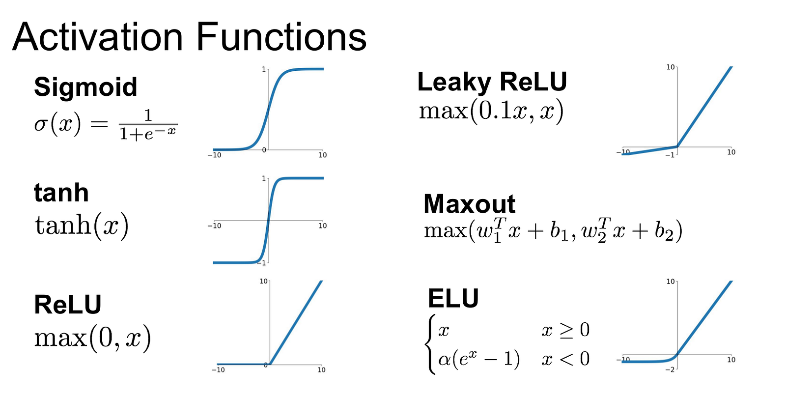
LeakyReLU is activation function. It is attempt to fix the “dying ReLU” problem.
In ReLU, if the input is not more than zero, weights can not change. So that, neurons become dead. With LeakyReLU, even if input is not more than zero, model can update weights. Thus, it become alive.
-
Batch Normalization means that normalize each batch by both mean and variance. (More information)
-
Dropout is a regularization technique. The key idea is to randomly drop units (along with their connections) from the neural network during training. This prevents units from co-adapting too much. This significantly reduces overfitting and gives major improvements over other regularization methods. (More information)
We are using LeakyReLU, BatchNormalization and Dropout for better generalization.
- Dense (Fully-Connected) layer implements the operation:
output = activation(dot(input, kernel) + bias)
We should compile this model. So that, we need tune two things.
- Optimizer
- Loss Function
I have used Stochastic Gradient Descent (SGD) for optimizer and categorical cross entropy for loss function.
-
Basically, in SGD, we are using the cost gradient of 1 example at each iteration, instead of using the sum of the cost gradient of ALL examples. (We update the weights after each training sample in SGD.)
-
In this example, we use categorical cross entropy for multi-class problem. Also, we use this type of loss function when we use softmax and one-hot encoded target.
-
We use cross-entropy to understand how predicted distribution differs from true distribution in real life applications with this formula.
- As you can expect, if cross-entropy (loss) decrease with updates of weights and biases, we can say predicted distribution better represent the true distribution. Thus, gradient based updates’ aim is decrease cross-entropy.
-

optimizer = keras.optimizers.SGD(lr=0.01)
model.compile(loss='categorical_crossentropy', optimizer=optimizer)
Training and Generation
Now, when we feed our deep learning model with training data, it predict same values. We use these values to sample. This part is a litte bit confusing. I have tried different methods. For instance, assume argument of max value as first touch and second max argument as continuation, however, it can not creates enjoyable music. So that, I have used this function.
def sample(preds, temperature=1.0):
    preds = np.asarray(preds).astype('float64')
    preds = np.log(preds) / temperature
    exp_preds = np.exp(preds)
    preds = exp_preds / np.sum(exp_preds)

    num_of_top = 15
    num_of_first = np.random.randint(1,3)


    preds [0:48] = 0 # eliminate notes with low octaves
    preds [100:] = 0 # eliminate notes with very high octaves

    ind = np.argpartition(preds, -1*num_of_top)[-1*num_of_top:]
    top_indices_sorted = ind[np.argsort(preds[ind])]


    array = np.random.uniform(0.0, 0.0, (128))
    array[top_indices_sorted[0:num_of_first]] = 1.0
    array[top_indices_sorted[num_of_first:num_of_first+3]] = 0.5

    return array
Now we can train our model. When our model is trained, we can create matrix. After that we can generate .mid with this matrix.
import random
import sys

epoch_total = 81
batch_size = 2

for epoch in range(1, epoch_total):
    print('Epoch:', epoch)
    model.fit(previous_full, predicted_full, batch_size=batch_size, epochs=1,
              shuffle=True)

    start_index = random.randint(0, len(midis_array)- max_len - 1)

    generated_midi = midis_array[start_index: start_index + max_len]


    if ((epoch%10) == 0):
      model.save_weights('my_model_weights.h5')

      for temperature in [1.2]:
          print('------ temperature:', temperature)

          for i in range(480):
              samples = generated_midi[i:]
              expanded_samples = np.expand_dims(samples, axis=0)
              preds = model.predict(expanded_samples, verbose=0)[0]
              preds = np.asarray(preds).astype('float64')

              next_array = sample(preds, temperature)

              midi_list = []
              midi_list.append(generated_midi)
              midi_list.append(next_array)
              generated_midi = np.vstack(midi_list)

          generated_midi_final = np.transpose(generated_midi,(1,0))
          output_notes = matrix_to_midi(generated_midi_final, random=0)
          midi_stream = stream.Stream(output_notes)
          midi_stream.write('midi', fp='lstm_output_v1_{}_{}.mid'.format(epoch, temperature))
DL models create matrix as output. We need convert this matrix to midi for listening. Now, let’s build matrix_to_midi function for this conversion.
- First read the matrix. (I have provide small part of codes. Because codes are too long to read in blogpost)
for y_axis_num in range(y_axis):
        one_freq_interval = matrix[y_axis_num,:] # values in one column
        one_freq_interval_norm = converter_func(one_freq_interval) # normalize values
        i = 0
        offset = 0

        if (random):

          while (i < len(one_freq_interval)):
              how_many_repetitive = 0
              temp_i = i
              if (one_freq_interval_norm[i] == first_touch):
                  how_many_repetitive = how_many_repetitive_func(one_freq_interval_norm, from_where=i+1, continuation=continuation)
                  i += how_many_repetitive

              if (how_many_repetitive > 0):
                  random_num = np.random.randint(3,6)
                  new_note = note.Note(int_to_note(y_axis_num),duration=duration.Duration(0.25*random_num*how_many_repetitive))
                  new_note.offset = 0.25*temp_i*2
                  new_note.storedInstrument = instrument.Piano()
                  output_notes.append(new_note)
              else:
                  i += 1

        else:

          while (i < len(one_freq_interval)):
              how_many_repetitive = 0
              temp_i = i
              if (one_freq_interval_norm[i] == first_touch):
                  how_many_repetitive = how_many_repetitive_func(one_freq_interval_norm, from_where=i+1, continuation=continuation)
                  i += how_many_repetitive

              if (how_many_repetitive > 0):
                  new_note = note.Note(int_to_note(y_axis_num),duration=duration.Duration(0.25*how_many_repetitive))
                  new_note.offset = 0.25*temp_i
                  new_note.storedInstrument = instrument.Piano()
                  output_notes.append(new_note)
              else:
                  i += 1

    return output_notes
Note: I have added some randomness to this conversion. If I do not use this randomness, length of notes will mostly become 0.25 because of model. Thus, generated music can not be enjoyable without this randomness.
As you can see, there is some function in this code. Now, look these functions.
- Converter_func is for give unique numbers to represent first touch, continuation and rest. If you use range for represent these values at midi_to_matrix you need this function.
def converter_func(arr,first_touch = 1.0, continuation = 0.0, lower_bound = lower_bound, upper_bound = upper_bound):
    # first touch represent start for note, continuation represent continuation for first touch, 0 represent end or rest
    np.place(arr, arr < lower_bound, -1.0)
    np.place(arr, (lower_bound <= arr) & (arr < upper_bound), 0.0)
    np.place(arr, arr >= upper_bound, 1.0)
    return arr
- how_many_repetitive_func is used to understand duration of note.
def how_many_repetitive_func(array, from_where=0, continuation=0.0):
    new_array = array[from_where:]
    count_repetitive = 1
    for i in new_array:
        if (i != continuation):
            return (count_repetitive)
        else:
            count_repetitive += 1
    return (count_repetitive)
Results
Let’s listen some outputs of the system.
I have used 55 different piano music for game for these outputs. I have trained my model 15 hours with Google Colab.
I want to say thanks to Oguzhan Ergin for his support.